- Learners can apply functions from the tidyr R Package to transform their data from a wide to a long format and vice versa.
- Learners can apply functions from the dplyr R Package to join multiple data sets.
- Learners can understand the relevance a data dictionary to describe variable names in a data set.
Pivoting & Joining & Metadata
ds4owd - data science for openwashdata
2023-12-12
Pivoting data
How would you plot this?
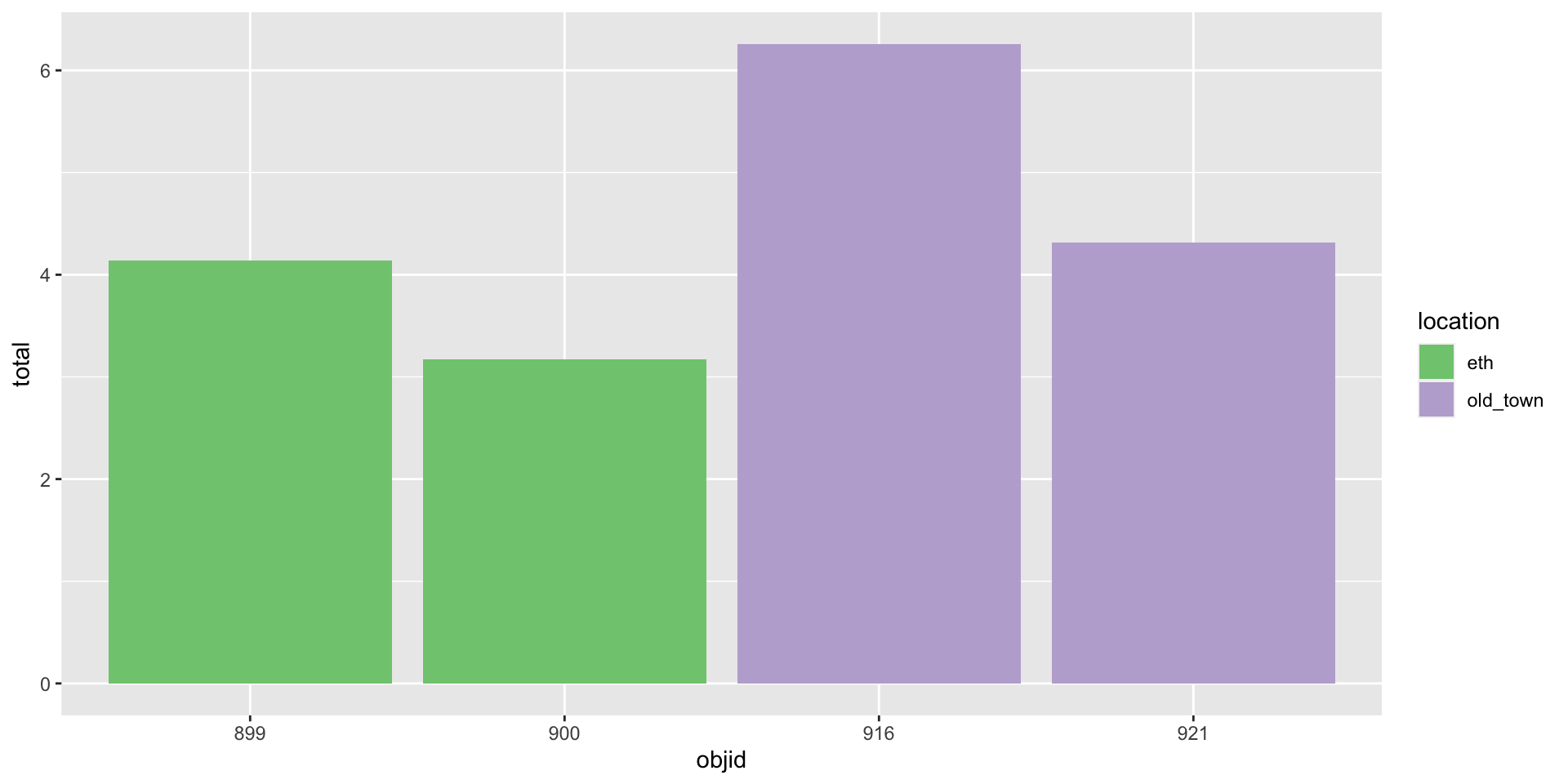
Three variables -> three aesthetics

And how to plot this?

Three variables -> three aesthetics
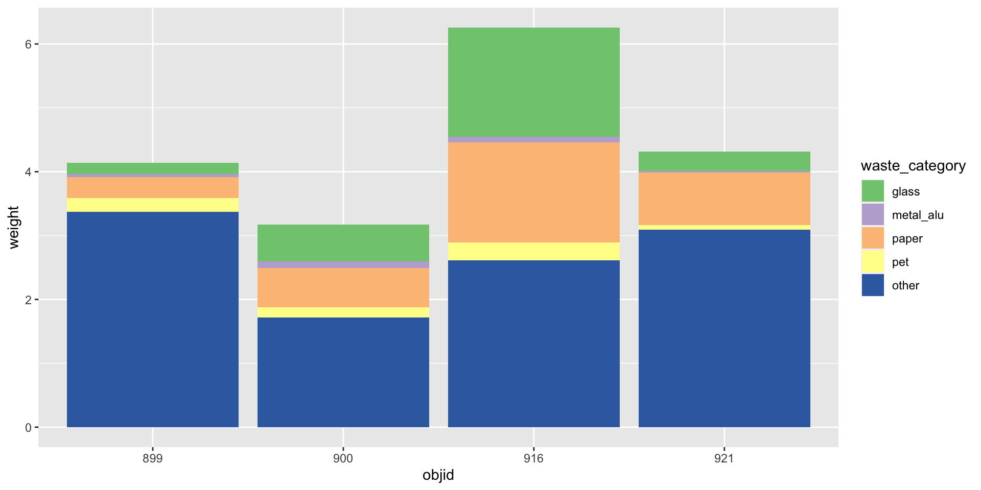
Three variables -> three aesthetics

Take a break
Please get up and move! Let your emails rest in peace.
10:00
left_join()

right_join()
full_join()

Faecal sludge samples
You download the XLSX file that contains the data and you open it in Excel. You see the following:
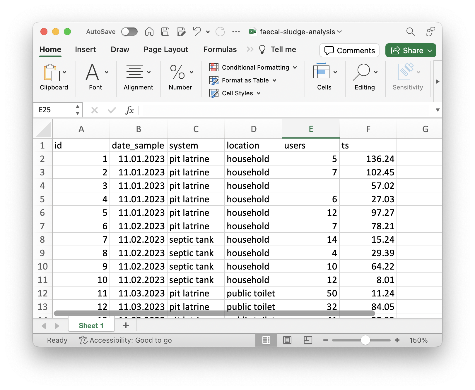
Faecal sludge samples
Open questions:
- What unit does
usersrefer to? - What does
tsstand for? - The
dateof what? - Where was this data collected?
- Which method was used to collect the samples?
Questions that only the original author may have the answers to.
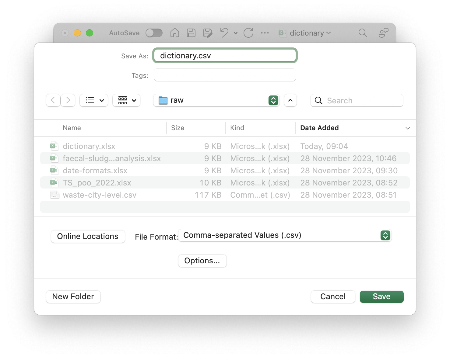
Data dictionary for faecal sludge samples
- Edit in spreadsheet software (e.g. MS Excel)

Data dictionary for faecal sludge samples
- Save as CSV file
Christmas break
- Lars will be on vacation from December 22nd until January 15th
- Mian and Sophia will be on vacation from December 22nd until January 8th

First lecture of 2024
Tuesday, January 16th at 2 pm CET

References
All material is licensed under Creative Commons Attribution Share Alike 4.0 International.
![]()
Wilson, Greg, Jennifer Bryan, Karen Cranston, Justin Kitzes, Lex Nederbragt, and Tracy K. Teal. 2017. “Good Enough Practices in Scientific Computing.” PLOS Computational Biology 13 (6): e1005510. https://doi.org/10.1371/journal.pcbi.1005510.